Basic Tutorial

The thevenin package is built around the following main classes:

1. Simulation and Predction - used to construct instances of an equivalent circuit model. The two interfaces are optimized for full timeseries simulations and step-by-step predictions, respectively.

2. Experiment - used to define an experimental simulation protocols containing current, voltage, and/or power-controlled steps.

3. StepSolution and CycleSolution - the result objects that contain simulation outputs when a particular simulation runs a particular experiment.

4. TransientState - a helper class to assist the user in managing the input and output states needed to interface with the Prediction class.

Each of these classes exist at the base package level so they are easily accessible. In this tutorial you will be introduced to each class through a minimal example. The example will demonstrate a typical workflow for constructing a model, defining an experiment, and interacting with the solution.

Construct a Simulation

The model class is constructed by providing options and parameters that define your circuit. The input can be given as either a dictionary or using a .yaml file. If you do not give an input, we include a default parameters file for you to get started. However, it is important that you understand this file and/or its dictionary equivalent so you can modify parameter definitions as necessary later. For more information about constructing model inputs, see the examples section.

Here, we will start by simply using the default parameters. A warning will print when the default parameters are accessed, but we can ignore it. After initialization, the class can be printed to check all of the constant options/parameters. The model also contains functional parameters, i.e., properties that change as a function of state of charge (SOC) and/or temperature. These values are difficult to represent in the printed output so they are not displayed.

import thevenin as thev

sim = thev.Simulation()
print(sim)

Simulation(
    num_RC_pairs=1,
    soc0=1.0,
    capacity=75.0,
    ce=1.0,
    gamma=0.0,
    mass=1.9,
    isothermal=False,
    Cp=745.0,
    T_inf=300.0,
    h_therm=12.0,
    A_therm=1.0,
)

[thevenin UserWarning] Using the default parameter file 'params.yaml'.

Options and parameters can be changed after initialization by modifying the corresponding attribute. However, if you modify anything after initialization, you should ALWAYS run the preprocessor pre() method afterward. This method is run automatically when the class is first initialized, but needs to be run again manually in some cases. One such case is when options and/or parameters are changed. Forgetting to do this will cause the internal state and options to not be self consistent. We demonstrate the correct way to make changes below, by setting the isothermal option to True.

sim.isothermal = True 
sim.pre()

Define an Experiment

Similar to how a typical battery cycler would be programmed, experiments are constructed by defining a series of sequential steps. Each step has its own mode (current, voltage, or power), value, time span, and limiting criteria.

While we will not cover options for the underlying solver in this tutorial, you should know that these options exist and are controlled through the Experiment class. Solver settings that should be consistent throughout all steps should be set with keyword arguments when the class instance is first created. You can also modify solver options at the per-step level (e.g., tighter tolerances) if needed. For more information, see the full documentation.

Below we construct an experiment instance with two simple steps. The first step discharges the battery at a constant current until it reaches 3 V. Afterward, the battery rests for 10 minutes. Note that the sign convention for current and power are such that positive values discharge the cell and negative values charge the cell.

expr = thev.Experiment()
expr.add_step('current_A', 75., (4000., 60.), limits=('voltage_V', 3.))
expr.add_step('current_A', 0., (600., 60.))

There are also control modes available for both voltage and power, and while we do not demonstrate it here, the load value does not need to be constant. You can run dynamic profiles during a step by passing in a callable value, like f(t: float) -> float, where t is the relative time (in seconds) for the step and the return value is the load at that time.

Pay attention to two important details in the example above:

1. The tspan input (third argument) uses 4000 seconds in the first step even though the current is chosen such that the battery should dischange within an hour. When the limits keyword argument is used in a step, and you want to guarantee the limit is actually reached, you will need to pick a time beyond when you expect the limiting event to occur.

2. The value 60. in the second position of the tspan argument contains a trailing decimal on purpose. When the decimal is present, Python interprets this as a float rather than an integer. The time step behavior is sensitive to this. When a float is passed, the solution is saved in intervals of this value (here, every 60 seconds). If an integer is passed instead, the full timespan is split into that number of times. In otherwords, dt = tspan[0] / (tspan[1] - 1). We recommend always use floats for steps that have limits.

Run the Simulation

The Simulation class contains two methods to run an experiment. You can either run the entire series of experiment steps by calling run(), or you can run one step at a time by calling run_step(). The most important difference between the two is that the model’s internal state is changed and saved at the end of each step when using run_step() so that it is ready for the following step. Therefore, steps should only ever be run in sequential order, and steps between multiple experiments should not be mixed. For example, to run the above two steps, one at a time, execute the following code.

soln_0 = sim.run_step(expr, 0)
soln_1 = sim.run_step(expr, 1)

Indexing starts at zero to be consistent with the Python language. When steps are run one at a time, the return value is a StepSolution instance, which we discuss below.

The most important thing to be aware of when running multiple steps or even multiple experiments is how the model stores and updates its internal state. When using run_step(), the model’s internal state is always saved at the end of each step. Therefore, each subsequent step starts off exactly where the previous step left off. The user can reset the model back to a rested condition at any point by manually calling the pre() method. A call to run() operates a bit differently.

The default behavior for run() will automatically run all steps in sequential order AND will reset the model state back to a rested condition at the of of the experiment. This is convenient for cases where you want to test discharge behaviors at different rates without needing to add charges in between each discharge. Using the default behavior, the model would simply start each discharge experiment from the same original rested state. You can bypass the state reset by using the optional reset_state=False keyword argument. Bypassing this reset is necessary if you plan to run sequential experiments in which the final battery state from a previous experiment needs to match the initial state of a following experiment. We also provide a way to initialize the battery state according to a previous solution by using the pre() method. See the full documentation for more information.

Below, we simply reset the model back to a rested condition since it was already run in the blocks above. After the pre-processing reset, we run both steps from the experiment defined above in one call to run(). Note that the solutions returned from the run() method are CycleSolution instances, which differ from StepSolution in some key ways. The following section comments on both types of solutions.

sim.pre()

soln = sim.run(expr)

Interacting with Solutions

Simulation outputs will give one of two solution objects depending on your run mode. A StepSolution is returned when you run step by step and a CycleSolution is returned when using run(). The latter simply stitches together the individual step solutions. Each solution object has numerous attributes to inform the user whether or not their simulation was successful, how long the integrator took, etc. For CycleSolution instances, most of the values are lists and the indices correspond to the steps from the experiment. For example, below we see that both steps were successful and the total integration time.

print(soln)

CycleSolution(
    solvetime=0.018 s,
    success=[True, True],
    status=[2, 1],
    nfev=[231, 67],
    njev=[31, 26],
    vars=['time_s', 'time_min', 'time_h', 'soc', 'temperature_K', 'voltage_V',
          'hysteresis_V', 'current_A', 'power_W', 'eta0_V', 'eta1_V'],
)

Most likely, everything else you will need to extract from solutions can be found in the solution’s vars dictionary. This dictionary contains easy to read names and units for all of the model’s outputs. You can check the available keys by printing the solution instance, as shown above.

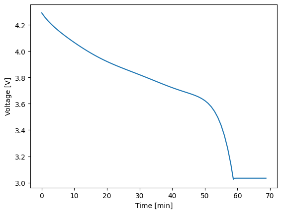
All values in the vars dictionary are 1D arrays that provide the values of the named variable at each integrator step. You can plot any two variables against each other using the plot() method. For example, the following code block plots the cell voltage against time.

soln.plot('time_min', 'voltage_V')

It is sometimes useful to extract portions of a CycleSolution to examine what occurred within a given step, or to combine StepSolution instances for post-processing or plotting purposes. Both of these features are available, as demonstrated below.

soln_0 = soln.get_steps(0)
soln_1 = soln.get_steps(1)

soln = thev.CycleSolution(soln_0, soln_1)