1. YAML File Inputs

This basic example will walk you through understanding a few of the main classes required to build and exercise equivalent circuit models using this package. The classes as the Simulation, Experiment, and StepSolution or CylceSolution classes. Simulations hold parameters associated with defining the battery circuit, experiments list a series of sequential steps that define a test protocol or duty cycle, and the solution classes provide an interface to access, manipulate, and/or plot the solution.

Note that there are also classes specific to implementing step-by-step state predictions. Specifically, see the TransientState and Prediction classes if you are interested in this functionality. In this tutorial, however, we will only be working with the Simulation class to demonstrate how to run full timeseries simulations.

1.1. Import Modules

import numpy as np
import thevenin as thev

1.2. Construct a Simulation

The model class can be constructed using either a .yaml file or a dictionary that specifies all keyword arguments shown in the documentation (help(thev.Simulation)). A default .yaml file is read in when no input is provided. This is simply for convenience to help users get up and going as quickly as possible. However, you should learn how to write your own .yaml file or dictionary input if you would like to use this package to its fullest extent.

The .yaml format is very similar to building a dictionary in Python. You can access a list of the default files, load their contents, download the template to a local directory, or even just print the file using included templates functions. For example, below we get a list of the available example templates and print out the contents of the first one (named params.yaml).

templates = thev.list_templates()
print(templates, '\n\n')

thev.print_templates(templates[0])

['params.yaml'] 


==============================
params.yaml
==============================
num_RC_pairs: 1
soc0: 1.
capacity: 75.
gamma: 0.
ce: 1.
mass: 1.9
isothermal: False
Cp: 745.
T_inf: 300.
h_therm: 12.
A_therm: 1.
ocv: !eval | 
    lambda soc:   84.6*soc**7 - 348.6*soc**6 + 592.3*soc**5 - 534.3*soc**4 \
                + 275.*soc**3 - 80.3*soc**2 + 12.8*soc + 2.8
M_hyst: !eval |
    lambda soc: 0.
R0: !eval |
    lambda soc, T_cell: 1e-4 + soc/1e5 - T_cell/3e9
R1: !eval |
    lambda soc, T_cell: 1e-5 + soc/1e5 - T_cell/3e9
C1: !eval |
    lambda soc, T_cell: 1e2 + soc*1e4 + np.exp(T_cell/300.)

You can either copy this template and edit as needed, or even call thev.download_templates([path]) to download the example files into a given local directory. Note above that some of the parameters must be input as a Callable. You can see this in the ocv and in the resistor/capacitor values. It is important that the inputs of these functions have the correct order, i.e., f(soc: float) -> float for ocv and M_hyst, and f(soc: float, T_cell: float) -> float for the resistor/capacitor values. The inputs represent the state of charge (soc, -) and cell temperature (T_cell, K). The ocv and M_hyst outputs should have units of Volts, and resistor and capacitor outputs should be in Ohms and Farads, respectively. Since .yaml files do not natively support python functions, this package uses a custom !eval constructor to interpret functional parameters. The !eval constructor should be followed by a pipe | so that the interpreter does not get confused by the colon in the lambda expression. np expressions and basic math are also supported when using the !eval constructor.

Although this example only uses a single RC pair, num_RC_pairs can be as low as 0 and can be as high as \(N\). The number of defined Rj and Cj elements in the .yaml file should be consistent with num_RC_pairs. For example, if num_RC_pairs=0 then only R0 should be defined, with no other resistors or capacitors. However, if num_RC_pairs=3 then the user should specify R0, R1, R2, R3, C1, C2, and C3. Note that the series resistor element R0 is always included, even when there are no RC pairs.

Below, we construct a Simulation instance with the default parameters from the above .yaml file. Again, if no input is provided then the default will be loaded. A warning will print to make it clear that these default parameters are being used. You could also pass in the name of the default parameters file if you want to make it clear to yourself that the params.yaml file is being used. Alternatively, you can load the default parameters into a dictionary, modify it, and then use the modified example to construct your Simulation. This would be done using params = thev.load_templates('params.yaml').

sim = thev.Simulation()
print(sim)

Simulation(
    num_RC_pairs=1,
    soc0=1.0,
    capacity=75.0,
    ce=1.0,
    gamma=0.0,
    mass=1.9,
    isothermal=False,
    Cp=745.0,
    T_inf=300.0,
    h_therm=12.0,
    A_therm=1.0,
)

[thevenin UserWarning] Using the default parameter file 'params.yaml'.

As mentioned above, you can see that a warning printed to let us know that we are using the default parameters. This is to ensure users that have similarly named files are in fact running with their preferred inputs, rather than the defaults. For example, if the user has a local file named params.yaml, the package will take the default as its preference. To avoid this behavior, be sure to specify the local or absolute path, e.g., ./params.yaml, or simply rename your file.

In addition to constructing the Simulation instance, we also print a summary of its current parameter values. All of the Callables are neglected in the summary since it is more challenging to print them nicely, especially in cases where the functions are much more complex. Overally, however, you can see that the values which are included match those shown in the .yaml file.

1.3. Build an Experiment

Experiments are built using the Experiment class. An experiment starts out empty and is then constructed by adding a series of current-, voltage-, or power-controlled steps. Each step requires knowing the control mode/units, the control value, a relative time span, and limiting criteria (optional). Control values can be specified as either constants or dynamic profiles with sinatures like f(t: float) -> float where t is the relative time of the new step, in seconds. The experiment below discharges at a nominal 1C rate for up to 1 hour. A limit is set such that if the voltage hits 3 V then the next step is triggered early. Afterward, the battery rests for 10 min before charging at 1C for 1 hours or until 4.3 V is reached. The remaining three steps perform a voltage hold at 4.3 V for 10 min, a constant power profile of 200 W for 1 hour or until 3.8 V is reached, and a sinusoidal voltage load for 10 min centered around 3.8 V.

Note that the time span for each step is constructed as (tmax: float, dt: float) which is used to determine the time array as tspan = np.arange(0., t_max + dt, dt). You can also construct a time array given tspan: float which allows the solver to choose the time steps for you. Or, if you prefer to have more control you can construct any 1D np.array that starts at zero and is monotonically increasing and pass it as tspan instead. In this case, just make sure that the array has a length greater than two. If you pass an array like np.array([0., tmax]) then the behavior will be the same as tpsan: float, where the solver chooses time steps for you. To learn more about building an experiment, including which limits are allowed and/or how to adjust solver settings on a per-step basis, see the documentation help(thev.Experiment).

dynamic_load = lambda t: 10e-3*np.sin(2.*np.pi*t / 120.) + 3.8

expr = thev.Experiment(max_step=10.)
expr.add_step('current_A', 75., (3600., 1.), limits=('voltage_V', 3.))
expr.add_step('current_A', 0., (600., 1.))
expr.add_step('current_A', -75., (3600., 1.), limits=('voltage_V', 4.3))
expr.add_step('voltage_V', 4.3, (600., 1.))
expr.add_step('power_W', 200., (3600., 1.), limits=('voltage_V', 3.8))
expr.add_step('voltage_V', dynamic_load, (600., 1.))

1.4. Run the Experiment

Experiments are run using either the run() method, as shown below, or the run_step() method. To run the discharge first, perform an analysis, and then run a rest, etc. then you will want to use the run_step() method. Steps should always be run in order because the model’s state is always updated at the end of each step in preparation for the next step. At the end of all steps you can manually reset the model state back to a resting condition at soc0 using the pre() method.

The default behavior of run() handles all of this “complexity” for you. A single call to run() will execute all steps of an experiment in the correct order AND will call pre() at the end of all steps. To bypass the call to the pre-processor you can use the optional reset_state=False keyword argument. This is important if you need the model to run multiple experiments back-to-back and want the start of each experiment to be consistent with the end of the last experiment. In the case below, we use the default behavior and allow the state to reset back to a rested condition at the end of all steps.

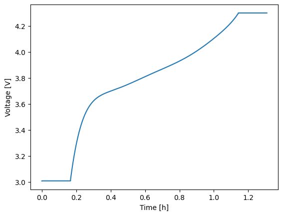
Regardless of how you run your experiment, the return value will be a solution instance. Solution instances each contain a vars attribute which contains a dictionary of the output variables. Keys are generally self descriptive and include units where applicable. To quickly plot any two variables against one another, use the plot method with the two keys of interest specified for the x and y variables of the figure. Below, time (in hours) is plotted against voltage.

soln = sim.run(expr)
soln.plot('time_h', 'voltage_V')

To run step-by-step, perform the following.

# Run each index, starting with 0
solns = []
for i in range(expr.num_steps):
    solns.append(sim.run_step(expr, i))
    
# Run the pre-processor to reset the state to a rested condition at soc0
sim.pre()
    
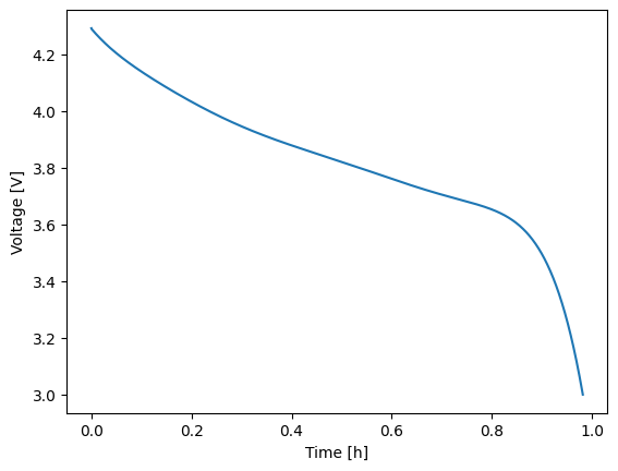
# Look at the first step solution (i.e., the 1C discharge)
solns[0].plot('time_h', 'voltage_V')

If you run an experiment step-by-step, you can also manually stitch them together into a CycleSolution once you are finished. Alternatively, if you have a CycleSolution, you can pull a single StepSolution or a subset of the CycleSolution using the get_steps method. See below for an example.

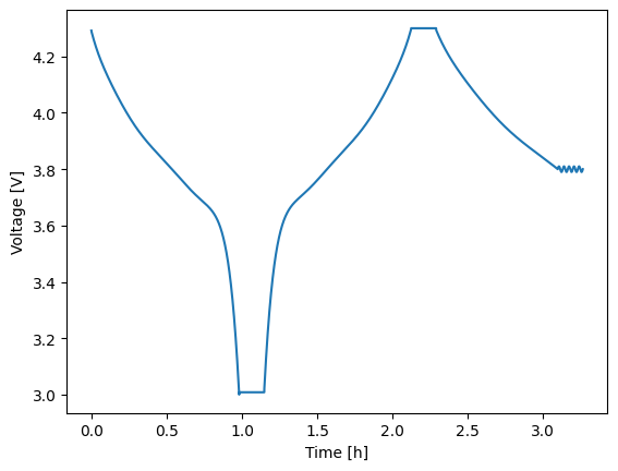
# Stitch the step solutions together
cycle_soln = thev.CycleSolution(*solns)
cycle_soln.plot('time_h', 'voltage_V')

# Pull steps 1--3 (inclusive)
some_steps = cycle_soln.get_steps((1, 3))
some_steps.plot('time_h', 'voltage_V')